epidemik

Compartmental Epidemic Models in Python

---

Table of contents

• Installation
• Tech Stack
• Features
• Basic Usage
• Network and metapopulation models
• Documentation
• Contributing
• License

---

Installation

Use the package manager pip to install epidemik. Python 3.8 or later is required.

pip install epidemik

To work on the package itself, clone the repository and let uv create the development environment (it installs the package in editable mode together with the test tools pinned in uv.lock):

git clone https://github.com/DataForScience/epidemik.git
cd epidemik
uv sync                 # add --group docs to also install Sphinx
uv run pytest           # run the test suite
uv build                # build the wheel and sdist

A plain pip install -e . also works if you prefer not to use uv.

[ ↑ Back to top ↑ ]

---

Tech Stack

Here's a brief high-level overview of the tech stack the epidemik package uses:

• The model is implemented as a directed multigraph using networkx
• Ordinary Differential Equations are numerically integrated using scipy
• Random numbers are generated by numpy
• Results are returned as pandas data frames
• Model structure visualizations rely on matplotlib
• Progress bars generated by tqdm

[ ↑ Back to top ↑ ]

---

Features

• Arbitrary compartmental models built from interaction (S + I -> I + I) and spontaneous (I -> R) transitions
• Named parameters that can be expressions of one another (mu="beta/2")
• Deterministic ODE integration and reproducible (seeded) discrete-time stochastic simulation with the same interface
• Generic computation of the basic reproduction number R₀ using the next-generation matrix
• Time-gated vaccination campaigns, birth and death rates, seasonal forcing
• Age structure driven by a contact matrix
• Multi-group (host/vector) models for vector-borne diseases and within-host (viral dynamics) models
• Epidemics on contact networks (NetworkEpiModel) and across coupled sub-populations (MetaEpiModel)
• Save and load model definitions as YAML files, and download ready-made models from the epidemik repository
• Quick plotting of trajectories and of the model structure itself

[ ↑ Back to top ↑ ]

---

Basic Usage

epidemik provides three main classes, EpiModel, NetworkEpiModel and MetaEpiModel, usually imported directly from the epidemik package

from epidemik import EpiModel

• EpiModel - Compartmental model in a homogeneously mixed population.
• NetworkEpiModel - Compartmental model on a network where nodes interact only along the edges connecting them.
• MetaEpiModel - Metapopulation model where sub-populations exchange individuals according to a travel matrix. Each sub-population has its own internal EpiModel instance.

To instantiate a new compartmental model we just need to create a EpiModel object and add the relevant transitions:

SIR = EpiModel(seed=42)
SIR.add_interaction('S', 'I', 'I', beta=0.2)
SIR.add_spontaneous('I', 'R', mu=0.1)

This fully defines the model. Rates are stored as named parameters (SIR.params) and may be expressions of one another, e.g. mu="beta/2". We can get a textual representation of the model using

print(SIR)

resulting in a YAML description of the model structure.

# Epidemic Model with 3 compartments and 2 transitions:

Compartments: [S, I, R]

Parameters:
  beta: 0.2
  mu: 0.1

Transitions:
  - S + I = I beta
  - I -> R mu

# R0=2.00

The same text can be written to a file with SIR.save_model("SIR.yaml") and read back with EpiModel.load_model("SIR.yaml"). A library of ready-made models can be listed with EpiModel.list_models() and fetched with EpiModel.download_model("SEIR.yaml").

or a graphical representation by calling draw_model():

SIR.draw_model()

The value of the Basic Reproduction Number (R₀) of the model can be determined using the R0() method:

SIR.R0()  # 2.0

There are two ways to explore the dynamics of the model, each with its corresponding method.

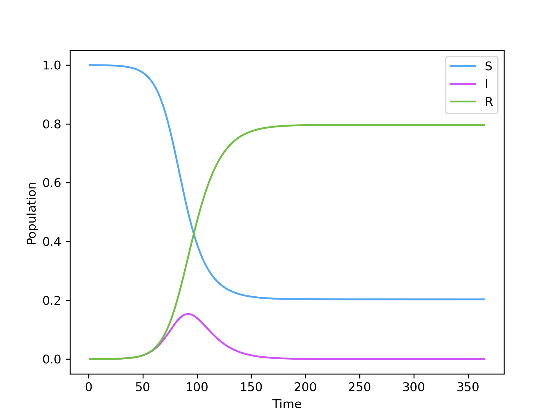
To integrate numerically the Ordinary Differential Equations that describe the model dynamics, we can call the integrate() method. The first argument is the number of time steps to integrate over and the remaining keyword arguments are the initial populations of each compartment.

N = 10_000
I0 = 10

SIR.integrate(365, S=N-I0, I=I0, R=0)

The results of the integration are stored in the values_ attribute as a pandas DataFrame indexed by time, whose first row holds the initial conditions. Individual compartments can be accessed as SIR.I or SIR[["S", "R"]]. A quick visualization of the results can be obtained using:

SIR.plot()

which produces:

To sample a single realization of the corresponding discrete-time stochastic process, call simulate() with the same arguments. The output has exactly the same shape and time index as the one produced by integrate():

SIR.simulate(365, S=N-I0, I=I0, R=0)
SIR.plot()

Vaccination campaigns, birth and death rates, seasonality, age structure and host/vector groups can be layered on top of any model:

SIR.add_vaccination("S", "V", rate=0.01, start=60)  # 1%/day, from day 60
SIR.add_birth_rate(0.0001, comps=["S"])             # newborns are susceptible
SIR.add_death_rate(0.0001)

vector = EpiModel()
vector.add_interaction("Sh", "Ih", "Iv", 0.3)   # Sh + Iv -> Ih + Iv
vector.add_interaction("Sv", "Iv", "Ih", 0.3)   # Sv + Ih -> Iv + Ih
vector.add_spontaneous("Ih", "Rh", 0.1)
vector.add_groups({"host": ["Sh", "Ih", "Rh"], "vector": ["Sv", "Iv"]})
vector.integrate(100, Sh=999, Ih=1, Rh=0, Sv=1000, Iv=10)

[ ↑ Back to top ↑ ]

---

Network and metapopulation models

NetworkEpiModel runs the same kind of model on top of a networkx graph, where each node is an individual that can only infect its neighbors. Simulations are seeded with a {node: compartment} dictionary:

import networkx as nx
from epidemik import NetworkEpiModel

G = nx.erdos_renyi_graph(1000, 0.01, seed=42)

net_SIR = NetworkEpiModel(G)
net_SIR.add_interaction("S", "I", "I", 0.05)
net_SIR.add_spontaneous("I", "R", 0.1)
net_SIR.simulate(100, seeds={0: "I", 1: "I"})

MetaEpiModel couples one EpiModel per sub-population through a row-stochastic travel matrix:

import pandas as pd
from epidemik import MetaEpiModel

travel = pd.DataFrame({"A": [0.99, 0.10], "B": [0.01, 0.90]}, index=["A", "B"])
populations = pd.DataFrame({"Population": [100_000, 10_000]}, index=["A", "B"])

meta_SIR = MetaEpiModel(travel, populations)
meta_SIR.add_interaction("S", "I", "I", 0.3)
meta_SIR.add_spontaneous("I", "R", 0.1)
meta_SIR.simulate(60, seed_state="A", I=10)

meta_SIR.get_state("B").plot()

[ ↑ Back to top ↑ ]

---

Documentation

The full documentation for this project is available at ReadTheDocs in html, PDF and ePub formats.

[ ↑ Back to top ↑ ]

---

Contributing

Pull requests are welcome. For major changes, please open an issue first to discuss what you would like to change.

Please make sure to update tests as appropriate. The test suite can be run with uv run pytest from the root of the repository.

Join our project and provide assistance by:

• Checking out the list of open issues where we need help.
• If you need new features, please open a new issue or start a discussion.

Contact us for the feedback or new ideas.

[ ↑ Back to top ↑ ]

---

Spread The Word

If you want to say thank you and/or support active development of the epidemik package:

• Add a GitHub star to the repository to encourage contributors and helps to grow our community.
• Tweet about the project on your Twitter!
  • Tag @data4sci and/or @bgoncalves

Thank you so much for your interest in growing our community!

---

License

epidemik is free and open-source software licensed under the MIT License [2024] - Bruno Gonçalves, Data For Science, Inc. Please have a look at the LICENSE.md for more details.

[ ↑ Back to top ↑ ]